Change-point models are a useful statistical tool for detecting change-points in time series data. Change-point models attempt to answer the question, “are there points in time when my data changes”?  The model will not only estimate the how the process changed (for example, went from a mean of 3 to a mean of 5), but also when these changes occurred. This is what makes these models so interesting- they quantify how and when a generative process changes over time.

How does it all work?   Like most statistical models, the likelihood explains a lot (if you’re not familiar with likelihood functions, this might be helpful). The likelihood helps us answer the question “what’s the probability of observing what I observed”?  Let’s look at the likelihood for a model with one change-point:

\[ \displaystyle L(Y)= \prod_{i=1}^{\tau}f_{0} (y) \prod_{i=\tau + 1}^{n} f_{1} (y) \]

The likelihood is made up of two products multiplied together: The first product quantifies the likelihood from the first point in our data, up to the change-point \( \tau \). The second product quantifies the likelihood from the change-point $ \tau $ to the end of our data. In this setup, the function $ f_{0} $ describes the data before the change-point, and the function $ f_{1} $ describes the data after the change-point. Once we have some data, we can use estimation methods to find the maximum likelihood estimators for $ \tau $, $ \mu $, and $ \sigma $.

Let’s look at an example to see how this really works.

Example In 1998, Massachusetts passed the nation’s toughest gun control legislation (you can find a summary of the legislation here). Did this legislation have any effect on gun-related deaths in Massachusetts? To find out, I used the CDC’s WONDER Database to find all gun-related deaths in Massachusetts from 1979 to 2015. Will a change-point model detect any change in the number of gun-related deaths? And if so, does the change line-up with the stricter gun-control legislation passed in 1998? Let’s find out!

To get a sense of the data, we can plot the number of gun-related deaths per million people for each year and add a lowess curve (trendline):

source: CDC WONDER Database

It looks like the number of gun-related deaths might have gone down after 1998, but it’s hard to tell. Let’s run our data through the change-point model. We can use the handy changepoint package in R:

# run change point model 
library(changepoint)
dat <-read.csv ( "gun_deaths.csv"; , stringsAsFactors = F)
dat$newrate <- dat$Deaths/dat$Population*1000000
mean.val <- cpt.mean (dat$newrate, method="AMOC"  )  
plot(mean.val ,  xaxt='n', xlab='Year', ylab='MA Gun Deaths per 1M People')

#print the change point and mean value estimates
cpts(mean.val)
summary(mean.val)
mean.val@param.est

Output:

summary(mean.val)

Created Using changepoint version 2.2.2 
Changepoint type      : Change in mean 
Method of analysis    : AMOC 
Test Statistic  : Normal 
Type of penalty       : MBIC with value, 10.83275 
Minimum Segment Length : 1 
Maximum no. of cpts   : 1 
Changepoint Locations : 17 

mean.val@param.est
$mean
[1] 46.17315 41.78381

Output graph:

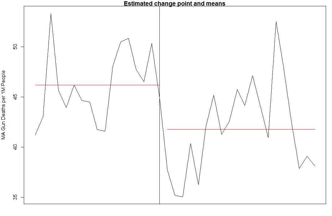
From looking at the graph and output, we can see the model estimated a change-point around time-point 17, which translates to 1996 in our data. The mean number of gun-related deaths before the change-point is estimated to be 46.2, and 42.2 afterwards.

So, did the 1998 gun-control legislation have an effect on the number of gun-related deaths? Well….maybe. Our model detected a change-point at 1996, two years before the legislation started. We can’t definitely say the legislation lowered the number of gun-related deaths, but we do see some evidence of a lower number of deaths after the legislation went into effect.